Descriptive Statistics
Descriptive statistics is the branch of statistics that involves summarizing and describing data using numerical calculations and graphical displays. It transforms raw numbers into meaningful insights that help us understand patterns, trends, and variability.
This guide covers key definitions, organizing data with histograms and frequency tables, measures of center and spread, five-number summaries, box plots, outlier detection, memory aids, and a practice quiz.
1Introduction
Have you ever looked at a huge table of numbers and felt overwhelmed? That is where descriptive statistics comes in. Descriptive statistics is the branch of statistics that involves summarizing and describing data using numerical calculations and graphical displays. It is about organizing, presenting, and interpreting data in a way that is easy to understand.
Understanding descriptive statistics is crucial because it allows us to make sense of information, identify patterns and trends, communicate findings effectively, and inform decisions using data.
Imagine you are a coach for a high school track team. You have just timed all 50 runners in the 100-meter dash. How do you figure out who the fastest runners are, what the typical speed of your team is, or how spread out the abilities are? You use descriptive statistics! Calculate the average time, find the fastest and slowest times, see how spread out the times are, and create a histogram to visualize the distribution.
Why It Matters
Make Sense of Information
Turn complex datasets into simple, understandable summaries that reveal the story behind the numbers.
Identify Patterns & Trends
Spot what is common, what is unusual, and how things are changing over time.
Communicate Findings
Share insights with others using clear graphs, charts, and numerical summaries.
Inform Decisions
Use data to make better choices in business, science, government, and everyday life.
2Key Definitions
Data
A collection of facts, such as numbers, words, measurements, observations, or descriptions of things.
Population
The entire group of individuals or instances about whom we want to draw conclusions. It is the whole pie.
Sample
A subset of the population from which data is actually collected. It is a slice of the pie, used to learn about the whole.
Parameter
A numerical characteristic that describes a population. Think P for Parameter, P for Population.
Statistic
A numerical characteristic that describes a sample. Think S for Statistic, S for Sample.
Variable
A characteristic or attribute that can be measured or observed for each individual in a population or sample.
Quantitative Variable
A variable that can be measured numerically (e.g., height, age, number of siblings).
Qualitative Variable
A variable that describes a characteristic using categories or labels (e.g., hair color, gender).
Frequency
The number of times a particular value or category appears in a dataset.
Outlier
An observation point that is distant from other observations -- an unusually high or low value compared to the rest.
Distribution
The pattern showing how frequently each value or range of values occurs in a dataset.
3Organizing Data
Before we can analyze data, we often need to organize it in a way that makes patterns more visible. Two key tools are frequency tables and histograms.
Frequency Tables
A frequency table lists all the categories or values of a variable and the number of times each occurs. For quantitative data, values are often grouped into intervals or bins.
Example: Test Score Distribution
| Score Interval | Frequency |
|---|---|
| 50 -- 59 | 2 |
| 60 -- 69 | 5 |
| 70 -- 79 | 12 |
| 80 -- 89 | 8 |
| 90 -- 100 | 3 |
Histograms & Distribution Shapes
A histogram is a powerful way to visualize the distribution of quantitative data. The horizontal axis shows data values (often in intervals) and the vertical axis shows frequency. Unlike bar charts, the bars in a histogram touch each other to indicate continuous data.
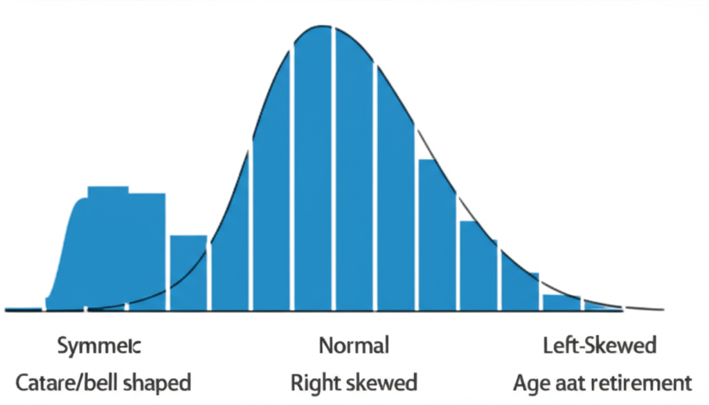
Symmetric
Left and right sides are approximate mirror images. Mean and median are roughly equal.
Skewed Left
Tail extends to the left. A few unusually low values pull the mean below the median.
Skewed Right
Tail extends to the right. A few unusually high values pull the mean above the median.
4Measures of Center
These statistics tell us about the "center" or typical value of a dataset. The three main measures are the mean, median, and mode.
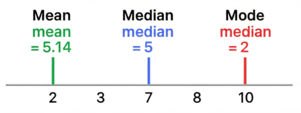
Mean (Arithmetic Average)
The mean is the sum of all values divided by the number of values. It is the most common measure of center but is sensitive to outliers.
x̄ = Σxᵢ / n
Sum of all data values divided by the number of values in the sample.
Median (Middle Value)
The median is the middle value when data is arranged in order. If n is odd, it is the single middle value. If n is even, it is the average of the two middle values. The median is resistant to outliers.
Mode (Most Frequent)
The mode is the value that appears most frequently. A dataset can be unimodal, bimodal, multimodal, or have no mode. The mode works for both quantitative and qualitative data.
When to Use Each
Mean
Best for symmetric distributions with no extreme outliers. Uses all data points.
Median
Best for skewed distributions or data with significant outliers. Resistant to extremes.
Mode
Useful for categorical data or finding the most common value. Works for any data type.
Worked Example: Mean, Median, Mode
Dataset: 10 quiz scores (out of 20)
Sorted: 10, 12, 14, 15, 16, 17, 18, 18, 19, 20
Mean
x̄ = 159 / 10
= 15.9
Median
n = 10 (even)
(16 + 17) / 2
= 16.5
Mode
18 appears twice
Mode = 18
5Measures of Spread
These statistics tell us how spread out or dispersed the data values are. A dataset can have the same center but very different spreads.
Range
Range = Maximum - Minimum
The simplest measure of spread. Easy to calculate but highly sensitive to outliers.
Interquartile Range (IQR)
IQR = Q3 - Q1
Measures the spread of the middle 50% of the data. Resistant to outliers.
Q1 (first quartile) is the median of the lower half of data (25th percentile). Q3 (third quartile) is the median of the upper half (75th percentile). When n is odd, do not include the overall median in either half.
Variance & Standard Deviation
Sample Variance
s² = Σ(xᵢ - x̄)² / (n - 1)
Average squared distance from the mean. Divide by n - 1 for unbiased estimation.
Sample Standard Deviation
s = √[Σ(xᵢ - x̄)² / (n - 1)]
Square root of variance. Same units as data, easier to interpret.
Worked Example: Standard Deviation
Data: 10, 12, 14, 15, 16, 17, 18, 18, 19, 20 | Mean (x̄) = 15.9 | n = 10
Step 1: Calculate deviations from mean
Step 2: Square each deviation
Step 3: Sum = 34.81 + 15.21 + 3.61 + 0.81 + 0.01 + 1.21 + 4.41 + 4.41 + 9.61 + 16.81
Σ(xᵢ - x̄)² = 90.9
s² = 90.9 / 9 = 10.1
s = √10.1 ≈ 3.178
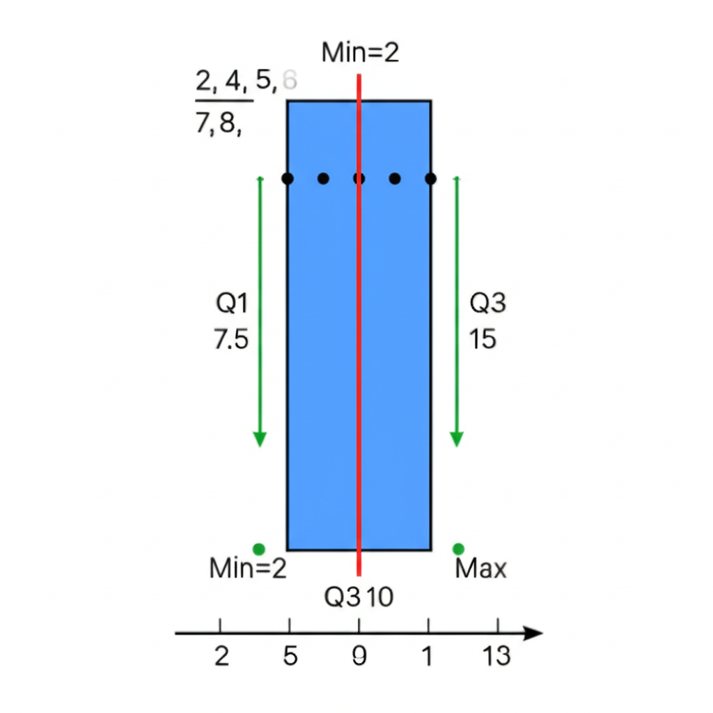
6Five-Number Summary & Box Plots
The five-number summary provides a concise description of a quantitative distribution using five key values.
Min
Smallest
Q1
25th %ile
Median
50th %ile
Q3
75th %ile
Max
Largest
Worked Example: Five-Number Summary
Sorted data: 10, 12, 14, 15, 16, 17, 18, 18, 19, 20
Minimum = 10
Lower half: 10, 12, 14, 15, 16 → Q1 = 14
Median = (16 + 17) / 2 = 16.5
Upper half: 17, 18, 18, 19, 20 → Q3 = 18
Maximum = 20
Five-Number Summary: 10, 14, 16.5, 18, 20
Constructing a Box Plot
Interactive: Box Plot Builder
Add or remove data points to see how the box plot, five-number summary, and outlier detection update in real-time.
Five-Number Summary
Sorted Data
12, 15, 18, 22, 25, 28, 30, 35, 42
- Draw a number line that covers the full range of your data.
- Draw a box from Q1 to Q3.
- Draw a line inside the box at the median.
- Draw whiskers from Q1 to the minimum and from Q3 to the maximum (or to the most extreme non-outlier values).
- Plot outliers individually as dots beyond the whiskers.
7Identifying Outliers
Outliers are identified using the 1.5 x IQR rule. Any value outside the calculated boundaries is considered a suspected outlier.
Lower Bound
Q1 - (1.5 × IQR)
Any value below this is a suspected outlier.
Upper Bound
Q3 + (1.5 × IQR)
Any value above this is a suspected outlier.
Worked Example: Outlier Detection
Using our dataset: Q1 = 14, Q3 = 18, IQR = 4
Lower Bound = 14 - (1.5 × 4) = 14 - 6 = 8
Upper Bound = 18 + (1.5 × 4) = 18 + 6 = 24
Data: 10, 12, 14, 15, 16, 17, 18, 18, 19, 20
Any values below 8? No. Any values above 24? No.
No outliers in this dataset.
8Memory Aids
"P for Population, P for Parameter; S for Sample, S for Statistic."
Helps remember that parameters describe populations and statistics describe samples.
"SKEW is where the TAIL is."
If the tail goes right, it is skewed right. If the tail goes left, it is skewed left. The mean is pulled in the direction of the tail.
"Min-Q1-Med-Q3-Max"
Think of it like a journey: start at the Minimum, pass the first quarter mark (Q1), hit the Median halfway point, reach the three-quarter mark (Q3), and arrive at the Maximum.
"IQR is the Inner Quarter Range."
Helps remember that IQR covers the middle 50% of the data, between the 25th and 75th percentiles.
"Standard Deviation is the Square Root of the Variance."
Helps remember the relationship and that standard deviation is in the original units of the data.
"Median for Skewed, Mean for Symmetric."
When data is skewed or has outliers, use the median and IQR. When data is symmetric, use the mean and standard deviation.
9Common Mistakes
Confusing mean and median
Using the mean when the data is heavily skewed or contains outliers, leading to a misleading representation of the center. Remember: median for skewed, mean for symmetric.
Incorrect outlier identification
Forgetting the 1.5 x IQR rule or applying it incorrectly. Always calculate Q1 - 1.5(IQR) and Q3 + 1.5(IQR) as your boundaries.
Misreading histogram shapes
Confusing a histogram with a bar chart (histograms are for quantitative data with touching bars). Also, misidentifying skewness -- the "tail" determines the direction of skew, not the peak.
Calculation errors for quartiles
When n is odd, including the median in both the lower and upper halves when calculating Q1 and Q3. The overall median should not be included in either half.
Forgetting n - 1 for sample standard deviation
Dividing by n instead of n - 1 for sample standard deviation or variance, leading to an underestimation. This is a crucial distinction between sample and population formulas.
Not sorting data first
Attempting to find the median or quartiles without first sorting the data in ascending order. This will always lead to incorrect results.
Misinterpreting standard deviation
Thinking a large standard deviation means the data values are all large, rather than meaning they are widely spread out from the mean.
Ignoring context
Presenting numerical summaries or graphs without discussing what they mean in the context of the problem. Always relate your findings back to the real-world scenario.
Quick Revision Summary
- ✓Descriptive statistics summarizes and describes data using numbers and graphs.
- ✓Parameters describe populations; statistics describe samples.
- ✓Variables can be quantitative (numerical) or qualitative (categorical).
- ✓Histograms display distribution shape: symmetric, skewed left, or skewed right.
- ✓Mean (average), median (middle, resistant to outliers), and mode (most frequent) measure center.
- ✓Range, IQR (resistant to outliers), variance, and standard deviation measure spread.
- ✓The five-number summary is Min, Q1, Median, Q3, Max -- visualized with a box plot.
- ✓Outliers are identified using the 1.5 x IQR rule: below Q1 - 1.5(IQR) or above Q3 + 1.5(IQR).
- ✓For skewed data, prefer median and IQR. For symmetric data, prefer mean and standard deviation.
- ✓Always sort data first before calculating median, quartiles, or the five-number summary.
Frequently Asked Questions
- What is the difference between a histogram and a bar chart?
- A histogram is used for quantitative (numerical) data, where the bars represent intervals of numbers and touch each other to show continuous data. A bar chart is used for qualitative (categorical) data, where each bar represents a distinct category and the bars typically do not touch.
- When should I use the mean versus the median?
- Use the mean for data that is relatively symmetric and does not have significant outliers, since it uses all data points. Use the median for skewed distributions or data that contains outliers, as the median is resistant to extreme values and better represents the "typical" value.
- Why do we divide by n - 1 instead of n for sample standard deviation?
- Dividing by n - 1 (called degrees of freedom) instead of n when calculating sample variance or standard deviation provides a more accurate, unbiased estimate of the population variance. If we used n, our sample statistic would tend to underestimate the true population parameter.
- What does a large standard deviation tell me?
- A large standard deviation means that the data points in your dataset are, on average, far away from the mean. This indicates a high degree of variability or spread in the data. Conversely, a small standard deviation means data points are clustered closely around the mean.
- How do I handle outliers once I have identified them?
- First, investigate whether the outlier is a data entry error, measurement error, or a legitimate but unusual value. Always report the presence of outliers and their potential impact. Depending on the context, you might remove erroneous values, analyze the data with and without the outlier, or use resistant measures like the median and IQR that are less affected by extreme values.
Practice Quiz
Test your understanding — select the correct answer for each question.
1.Which measure of center is best for data with outliers?
2.What does the IQR represent?
3.A histogram shows:
4.The mode is:
5.Standard deviation measures:
6.Q3 is also called:
7.An outlier is defined as:
8.The five-number summary includes:
9.A right-skewed distribution has:
10.Variance is:
Final Study Advice
- 1.Always sort your data before calculating any positional statistics (median, quartiles, percentiles).
- 2.Choose the right measure of center: mean for symmetric data, median for skewed data or data with outliers.
- 3.Practice drawing box plots from five-number summaries -- they appear frequently on exams.
- 4.Remember to divide by n - 1 (not n) when calculating sample variance and standard deviation.
- 5.Always interpret your results in context -- relate numbers back to what the data represents in the real world.